相关度算法背后的理论知识
Lucene 包括 Elasticsearch 使用 “布尔模型” 来搜索相关的文档,然后使用“真实的计分函数”来计算相关度评分。而这个计分函数又引入了“TF/IDF”和“向量空间模型”的概念,并提供了一些更先进的功能,比如增加了一个协调因子,字段长度规整化功能以及词元或查询子句加权降权的功能。
Note
小伙子,别方!这些概念听上去很唬人,但其实并不难理解。本章节提交的很多概念性的诸如算法,公式,数学建模等知识,虽然都是前人总结出来给其他人看的,但其实理解这些知识点本身,并没有直接去理解有哪些因素会影响最终的相关度得分来得重要。
布尔模型
所谓布尔模型,就是用与,或,非条件来表述一个查询条件。一个类似下面这样的查询条件:
full and text and search and (lucene or elasticsearch)
就只会搜索出含有“full”,“text”,以及“search”并且还含有“lucene”或者“elasticsearch”的结果。
词频/反转文档频率 TF/IDF这么学术的词汇应该有官方翻译版本吧。。。
看不懂翻译直接百度一下,很多博客有介绍什么是 TF/IDF
全文检索的结果集是需要按照相关度进行排序的。因为不是所有的结果都和查询条件完全匹配,而查询条件中的有的关键字又可能比其他关键字重要。(简单理解下,我搜“哪个网站适合装逼”,“网站”和“装逼”这两个词的重要性明显就比“哪个”,“适合”要重要的多,然后我就搜出了知乎。。。)某个搜索结果与查询条件之间的相关度部分会受到该结果中包含的部分“查询词”的影响。
我们之前在 What Is Relevance? 一文中介绍过,一个“查询词”(或者就直接叫词元吧)的权重取决于三点。也介绍了相应的计算的公式,但讲真,你没必要去记住那个公式,那只是写给感兴趣的人看的。
词频
词频用来表示搜索关键词中的某个词元在某个匹配到的文档中的出现频率。某个搜索关键词在某个被匹配到的文档中出现得越频繁,那么这个文档的相关度就越高。同一个词元在文档 A 中出现了 5 次,一般都比只出现了一次的文档 B 要高说一般是指不考虑有其他词元的时候。词频计算公式:
tf(t in d) = √frequency ①
① 词元(T term)词频(TF term frequence)
Theory Behind Relevance Scoring
Lucene (and thus Elasticsearch) uses the Boolean model to find matching documents, and a formula called the practical scoring function to calculate relevance. This formula borrows concepts from term frequency/inverse document frequency and the vector space model but adds more-modern features like a coordination factor, field length normalization, and term or query clause boosting.
Note
Don’t be alarmed! These concepts are not as complicated as the names make them appear. While this section mentions algorithms, formulae, and mathematical models, it is intended for consumption by mere humans. Understanding the algorithms themselves is not as important as understanding the factors that influence the outcome.
Boolean Model
The Boolean model simply applies the AND, OR, and NOT conditions expressed in the query to find all the documents that match. A query for
full AND text AND search AND (elasticsearch OR lucene)
will include only documents that contain all of the terms full, text, and search, and either elasticsearch or lucene.
This process is simple and fast. It is used to exclude any documents that cannot possibly match the query.
Term Frequency/Inverse Document Frequency (TF/IDF)
Once we have a list of matching documents, they need to be ranked by relevance. Not all documents will contain all the terms, and some terms are more important than others. The relevance score of the whole document depends (in part) on the weight of each query term that appears in that document.
The weight of a term is determined by three factors, which we already introduced in What Is Relevance?. The formulae are included for interest’s sake, but you are not required to remember them.
Term frequency
How often does the term appear in this document? The more often, the higher the weight. A field containing five mentions of the same term is more likely to be relevant than a field containing just one mention. The term frequency is calculated as follows:
tf(t in d) = √frequency ①
① The term frequency (tf) for term t in document d is the square root of the number of times the term appears in the document.
If you don’t care about how often a term appears in a field, and all you care about is that the term is present, then you can disable term frequencies in the field mapping:
PUT /my_index
{
  "mappings": {
    "doc": {
      "properties": {
        "text": {
          "type":          "string",
          "index_options": "docs" ①
        }
      }
    }
  }
}
① Setting index_options to docs will disable term frequencies and term positions. A field with this mapping will not count how many times a term appears, and will not be usable for phrase or proximity queries. Exact-value not_analyzed string fields use this setting by default.
Inverse document frequency
How often does the term appear in all documents in the collection? The more often, the lower the weight. Common terms like and or the contribute little to relevance, as they appear in most documents, while uncommon terms like elastic or hippopotamus help us zoom in on the most interesting documents. The inverse document frequency is calculated as follows:
idf(t) = 1 + log ( numDocs / (docFreq + 1)) ①
① The inverse document frequency (idf) of term t is the logarithm of the number of documents in the index, divided by the number of documents that contain the term.
Field-length norm
How long is the field? The shorter the field, the higher the weight. If a term appears in a short field, such as a title field, it is more likely that the content of that field is about the term than if the same term appears in a much bigger body field. The field length norm is calculated as follows:
norm(d) = 1 / √numTerms ①
① The field-length norm (norm) is the inverse square root of the number of terms in the field.
While the field-length norm is important for full-text search, many other fields don’t need norms. Norms consume approximately 1 byte per string field per document in the index, whether or not a document contains the field. Exact-value not_analyzed string fields have norms disabled by default, but you can use the field mapping to disable norms on analyzed fields as well:
PUT /my_index
{
  "mappings": {
    "doc": {
      "properties": {
        "text": {
          "type": "string",
          "norms": { "enabled": false } ①
        }
      }
    }
  }
}
① This field will not take the field-length norm into account. A long field and a short field will be scored as if they were the same length.
For use cases such as logging, norms are not useful. All you care about is whether a field contains a particular error code or a particular browser identifier. The length of the field does not affect the outcome. Disabling norms can save a significant amount of memory.
Putting it together
These three factors—term frequency, inverse document frequency, and field-length norm—are calculated and stored at index time. Together, they are used to calculate the weight of a single term in a particular document.
Tip
When we refer to documents in the preceding formulae, we are actually talking about a field within a document. Each field has its own inverted index and thus, for TF/IDF purposes, the value of the field is the value of the document.
When we run a simple term query with explain set to true (see Understanding the Score), you will see that the only factors involved in calculating the score are the ones explained in the preceding sections:
PUT /my_index/doc/1
{ "text" : "quick brown fox" }


GET /my_index/doc/_search?explain
{
  "query": {
    "term": {
      "text": "fox"
    }
  }
}
The (abbreviated) explanation from the preceding request is as follows:
weight(text:fox in 0) [PerFieldSimilarity]:  0.15342641 ①
result of:
    fieldWeight in 0                         0.15342641
    product of:
        tf(freq=1.0), with freq of 1:        1.0        ②
        idf(docFreq=1, maxDocs=1):           0.30685282 ③
        fieldNorm(doc=0):                    0.5        ④
① The final score for term fox in field text in the document with internal Lucene doc ID 0.
② The term fox appears once in the text field in this document.
③ The inverse document frequency of fox in the text field in all documents in this index.
④ The field-length normalization factor for this field.
Of course, queries usually consist of more than one term, so we need a way of combining the weights of multiple terms. For this, we turn to the vector space model.
Vector Space Model
The vector space model provides a way of comparing a multiterm query against a document. The output is a single score that represents how well the document matches the query. In order to do this, the model represents both the document and the query as vectors.
A vector is really just a one-dimensional array containing numbers, for example:
[1,2,5,22,3,8]
In the vector space model, each number in the vector is the weight of a term, as calculated with term frequency/inverse document frequency.
Tip
While TF/IDF is the default way of calculating term weights for the vector space model, it is not the only way. Other models like Okapi-BM25 exist and are available in Elasticsearch. TF/IDF is the default because it is a simple, efficient algorithm that produces high-quality search results and has stood the test of time.
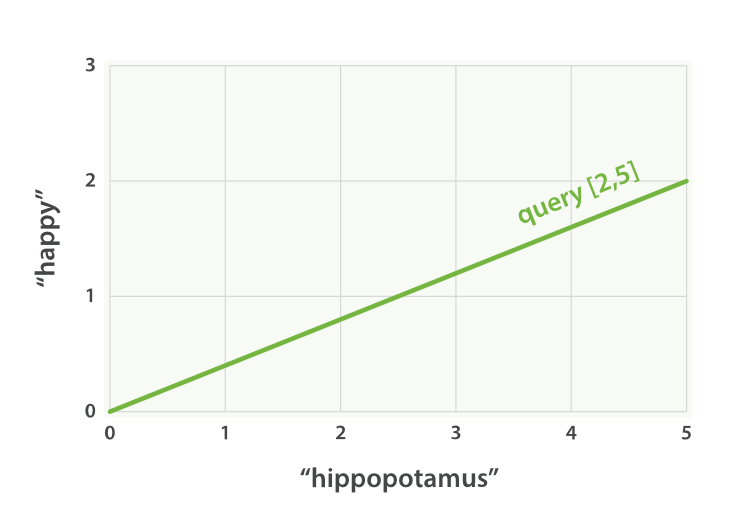
Imagine that we have a query for “happy hippopotamus.” A common word like happy will have a low weight, while an uncommon term like hippopotamus will have a high weight. Let’s assume that happy has a weight of 2 and hippopotamus has a weight of 5. We can plot this simple two-dimensional vector—[2,5]—as a line on a graph starting at point (0,0) and ending at point (2,5), as shown in Figure 27, “A two-dimensional query vector for “happy hippopotamus” represented”.
Figure 27. A two-dimensional query vector for “happy hippopotamus” represented
Now, imagine we have three documents:
- I am happy in summer.
- After Christmas I’m a hippopotamus.
- The happy hippopotamus helped Harry.
We can create a similar vector for each document, consisting of the weight of each query term—happy and hippopotamus—that appears in the document, and plot these vectors on the same graph, as shown in Figure 28, “Query and document vectors for “happy hippopotamus””:
- Document 1: (happy,___________)—[2,0]
- Document 2: (____ ,hippopotamus)—[0,5]
- Document 3: (happy,hippopotamus)—[2,5]
Figure 28. Query and document vectors for “happy hippopotamus”
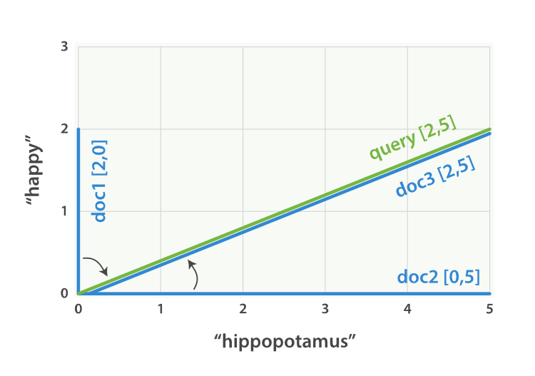
The nice thing about vectors is that they can be compared. By measuring the angle between the query vector and the document vector, it is possible to assign a relevance score to each document. The angle between document 1 and the query is large, so it is of low relevance. Document 2 is closer to the query, meaning that it is reasonably relevant, and document 3 is a perfect match.
Tip
In practice, only two-dimensional vectors (queries with two terms) can be plotted easily on a graph. Fortunately, linear algebra—the branch of mathematics that deals with vectors—provides tools to compare the angle between multidimensional vectors, which means that we can apply the same principles explained above to queries that consist of many terms.
You can read more about how to compare two vectors by using cosine similarity.
Now that we have talked about the theoretical basis of scoring, we can move on to see how scoring is implemented in Lucene.